Sums of Series: The Building Blocks

Sequences and series are an area of mathematics that often yield unexpected and possibly unintuitive results, a sequence being a collection of consecutive numbers which are related in some way, and a series being the sum of these numbers. Sigma notation is often used for the sum of a series, where the formula for values in the series, f(r) is given, and i is the start number to be put into the formula and n the final number, as below.

This can be a tool for many useful things, but here we are going to consider the functions n, n² and n³ as the result from these can be ascertained from physical demonstrations (though showing n³ requires an extra dimension), and they can be used to calculate a formula for any function that is a polynomial up to n³.

One of the most famous stories about these sums concerns the function n and Carl Friedrich Gauss, a mathematician and physicist who lived between 1777 and 1855. From an early age he was a great mathematician, and so when at school his teacher endeavoured to find things for him to do. One day, to keep him occupied, the teacher told him to add up all the numbers from 1 to 100, otherwise written as . Unfortunately for the teacher he had and answer in seconds: 5050. Instead of manually going through and adding all the numbers, he had realised that you can pair opposite ends of this series to 101 (100+1, 99+2, 98+3 etc.), and do so until you sum 50 and 51, which then gives you 50 lots of 101, or 5050. This was an ingenious way of finding the answer, but more to mathematicians a defined formula would be more useful. To do this one can quite simply turn to building blocks. The first step in this is to ask what sort of numbers you get for the first few values, which are 1, 3, 6, 10, 15, 21 and so on. This may or may not be familiar to you, but are in fact the triangle numbers, which makes sense when you think that when forming a triangle number you are adding a number one more than the previous number added. If we construct this for, say, the fourth triangle number 10, we will have as below.

We cannot ascertain a formula from this though as that is what we’re looking for in the first place. What if we add another triangle of the same size though? As can be seen below, we now have a rectangle of height 5 and length 4, or n×(n+1).

What then is the sum of one of the triangles, well it is 10, or ½n(n+1). This clearly works for all numbers n as every time you add one to n you add and extra row on each end, then move the top triangle right one and down one creating a rectangle of the above form. Hence we have a formula for .

What happens if we want to know the sum of a series of square numbers though? Well if we again consider this up to the fourth number we have a sequence of 1, 4, 9, 16. If we transfer these to physical blocks, we can see that these can be arranged to form a square-based pyramid, and their sums are square pyramidal numbers.

Now the question is how some number of these pyramids can be arranged into a cuboid with side lengths in terms of n. If we keep our first pyramid as shown above, the second one is arranged as below.

A third pyramid then  slots into the gap shown.

Another structure the same from the one above except with the left hand pyramid moved up and along and the right hand one moved right and down can then be put on top of this to form a cuboid.

Here we see 6 of the pyramids forming a structure of dimensions 4×5×9, and in a similar way to the two dimensional case above we can extend this finding to a general case where .

The formula for a sum of cubes, , is  . This can be ascertained by considering 4-dimensional pyramids formed of cubes of sidelength 1, 2, 3, … , n-2, n-1, n, but the human mind isn’t particularly adept at imagining the fourth dimension, so this method isn’t so useful, however the reverse process is something to think about. Here we see that 4 4D pyramids as described above can be arranged in such a manner that they produce a 4D cuboid of sidelengths n, n, n+1, and n+1. This can be taken up to any number of dimensions, where the xth dimension is used to find a formula for .

These results can be used for any polynomial up to a third order polynomial by simply splitting the polynomial into sums of cube values, square values, single values, and constants, however if a formula is produced in the same method in higher dimensions, results for higher order polynomials can be calculated, though that is rather a large if.

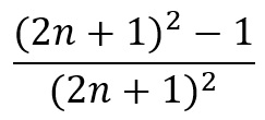
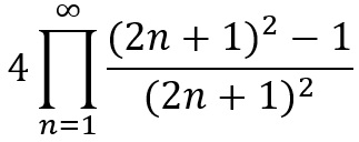
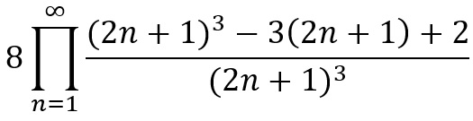
The Menger Sponge

Fractals have been touched upon previously regarding the Mandelbrot set, but here I want to introduce something a touch more simple. Imagine you have a square of card in front of you. Divide it into nine equal squares then punch out the central square. Now look at the remaining eight squares. Divide these into nine squares each, then punch out the central hole of each of these. Repeat this process again and again as your squares gradually get smaller then repeat this an infinite number of times. If you attempt this on a real piece of card you will find it soon becomes very difficult, or if you repeat as an animation, your initial square will soon seem to disappear. This is because your Sierpinski Carpet (the fractal was named after its founder in 1916) has no area, but does have an infinite perimeter. This is quite easy to see with only the smallest use of maths. Originally we had a square, we divided it into nine, then removed one of these nine (one ninth of the starting area) to leave eight squares (eight ninths of the starting area). We then repeat the process and take one ninth of all the remaining squares, so our square of one unit’s surface area was reduced to eight ninths of its size, and has been again. This repeats for every iteration you perform, and can be quite simply be written as

where n is the number of iterations carried out. I said above that we should carry this out an infinite number of times, and as your result gets smaller as n gets bigger, this tends to 0 as n tends to ∞. For each iteration the perimeter, on the other hand, has been increasing. For the first iteration we added four times a third of the original length of the square once, then we added four times a ninth of the original length eight times, then we added four times a twenty-seventh of the original length sixty-four times and so on, which can be summarised as below.

We can see that the numerator increases at a greater rate than the denominator, and so each consecutive term is larger, so both the terms and the overall sum tend to infinity.

This can be taken out of two dimensions as well. If we instead consider a cube, then divide it into 27 smaller cubes of equal dimensions to one another then punch the centre ones out as seen form each face so that there is a whole all of the way through the cube. As with the Sierpinski Carpet, we then repeat this process on the smaller cubes, and the process gradually produces the image below, a Menger Sponge.

This has the same properties as the Sierpinski Carpet, just in one higher dimension: the volume is equal to zero, and the surface area is infinite, and the same logic can be followed to deduce this, just with the volume changing by a factor of 20/27, and the surface area for each iteration is

and again as n tends to infinity, so will the surface area. Unfortunately it is quite hard to define an object that has infinite surface area and no volume, so things get a bit weird. It isn’t a 3D object as it has no volume, and if someone described an object that had no volume to you, you would probably say it was not 3D, even if the illustration of the Menger Sponge seems to contradict that. If, however, you choose one particular spot and looked at it, it will just be full of infinitely many holes, so appear to have no area (though the maths says otherwise) so it isn’t described as a 2D object either, instead its topological dimension is a 1D curve.

Many exciting things can come out of the Menger Sponge. If you were to look along the Menger Sponge’s diagonal, then make a perpendicular cut halfway along this line you will get a hexagonal fractal with repeating hexagrams (which look like six pointed stars).

Hexagonal Fractal

An even more exciting thing to get out of the Menger Sponge is pi. To explain this we have to start with the Sierpinski Carpet, as Ed Pegg, noted for being one of the first to do this, did. If you start with a square of 2 units by 2 units, divided into four smaller squares, you have a square of area 4 units squared. Now divide these four squares into 9 other squares and pop the central one out, then divide the resulting 32 squares not into 9 squares each but instead 25 squares and remove the centre square again. For each iteration the divisions on a length of one of the squares will increase by 2, so they will be an odd number in length, and that number squared for the area (3 and 9, then 5 and 25 above), as a proportion of the last iteration it will be the odd number squared minus one, divided by the odd number squared. Written more simply as

which will be 8/9 for the first iteration, then 24/25, then 48/49, then 80/81 and so on. Unlike a true Sierpinski Carpet the area of this does not tend to 0 as for each iteration the proportion of area removed decreases. Instead something far more exciting happens: the area tends towards pi! We can write the product as

which equals pi (though if infinity’s too big for consideration, replacing it with 100,000,000 gives 3.1415). What other shapes have a distance of one from their centre to their outside edge? The circle of course, which may seem irrelevant, but comes up quite surprisingly with the Menger Sponge. If we repeat the above process in 3 dimensions (it is three dimensions this time as some volume remains) we get the product equation

which gives 4π/3. Ring a bell? This is the volume of a sphere of radius one!

If this hasn’t all been quite exciting enough for you, you could instead make your own Menger Sponge. For the more casual mathematician you can visit http://megamenger.com/ to find the instructions for the construction of a first order Menger Sponge (mine is pictured below).

This was run by a group called Mega Menger who endeavoured to create a level 4 Menger Sponge distributed around the world, which meant creating 20 sponges (level 3) made of 20 smaller sponges (level 2), each made of 20 of the one pictured above (a level 1 sponge). A map of all the level 3 locations can be found on the Mega Menger website, but sites include the Cambridge University Maths Department, pictured badly below from my recent visit there; the University of Bath; Tampere, Finland; Almería, Spain; Dulwich International High School, Suzhou, China; and the Auckland Art Gallery, New Zealand.

Rather surprisingly of the great achievements of many of these institutions have produced, these level 3 Menger Sponges take pride of place in key areas of their buildings, for example in Cambridge it was only a few steps from the main door. So, if you want to do some not particularly taxing maths, remember even Cambridge maths students enjoy a bit of arts and crafts.

---

Update: Though the University of Bath did create a third order Menger Sponge it has since been destroyed due to irreparable wear and tear.

Projectiles on a Wobbly Plane

Many an A-Level mathematician or physicist will be familiar with the concept of projectile motion, being the description of how an object with negligible mass travels if the only force acting on it is gravity. This is a rare situation to come across in real life, especially when the person carrying out these calculations only ever considers the world as a big flat plane, where a projectile has travelled its maximum horizontal displacement for any given angle and initial velocity is when its vertical displacement is zero. If we take a step into the real(ish) world we will be hard pressed to find a large, very flat plane, which is why I thought it would be interesting to consider a more wobbly plane.

To start with I will describe how basic projectile motions are calculated (so if you already know about this, you can skip this paragraph). Two facts are normally known with a projectile, its initial velocity, and its angle to the horizontal, shown by v and θ below.

From this we can break the velocity into its components. What we effectively have here is a right-angled triangle, and we know cos(θ)=adjacent/hypotenuse, so adjacent=v×cos(θ), and sin(θ)=opposite/hypotenuse, so opposite=v×sin(θ). This can be written in column vector form as below.

Because of the above specified conditions (negligible mass; no force bar gravity), there is no accelerating or decelerating force horizontally, and there is an accelerative force downwards at 9.8ms^-2. At the furthest distance the vertical displacement equals zero, we know acceleration equals -9.8ms^-2 and the initial velocity is vsin(θ) ms^-1. To find the time for which the projectile travels we use the equation s=ut+0.5at² to obtain 0=t(vsin(θ)-4.9t). Thus t equals either 0 (when the projectile is at its start point) or vsin(θ)/4.9. Horizontally there is no acceleration, so the equation displacement equals velocity multiplied by time (s=vt) can be used, so the horizontal distance travelled equals v²sin(θ)cos(θ)/4.9.

This, however, is not the case if the plane is not flat, as the ground will be moving relative to the projectile, so the below equation needs resolving.

This equation seems a bit random, so we first need to know what all of the symbols stand for. α is the angle that the projectile is being fired at relative to the surface on which it sits (aka the tangent to the curve), θ is the angle of the surface relative to the horizontal (at the point of firing, where horizontal displacement equals zero), v is the initial velocity, and the function f(x) is the equation  of the surface. x is the horizontal distance that needs resolving.

To find the angle θ we need to know the gradient of the tangent to the curve which touches the curve when x equals zero. To do this we simply find the derivative of the curve at zero, written as f´(x). A gradient is equal to the change in vertical (y) units divided by the change in horizontal (x) units, and tan(θ) is equal to opposite/adjacent in a right-angled triangle, or on the graph above the change in vertical units divided by the change in horizontal units, so tan(θ)=f´(x), so θ=arctan(f´(0)). Now that we know this we can work out the angle at which the projectile is fired relative to the horizontal: (α-arctan(f´(0)))­º. We can split the initial velocity into components now:

As established velocity=displacement/time, so horizontally time=displacement/velocity, so t=x/(vcos(α-arctan(f´(0)))). Using the SUVAT equations of motion (specifically s=ut+0.5at²), we know that the vertical displacement equals vcos(α-arctan(f´(0)))t – 4.9t². Substituting in our equation for t in terms of x, v, and α we have (vcos(α-arctan(f´(0)))x)/(vcos(α-arctan(f´(0)))) – 4.9 (x/(vcos(α-arctan(f´(0))))², which can be written as:

The projectile will have landed when its vertical displacement is the same as the vertical displacement of the surface for the same value of x, so we just equate the above to f(x), then account for the fact that the projectile may not be ejected from a vertical displacement of zero by adding f(0) (the vertical displacement of the surface relative to the origin at zero displacement), and we can see how far the projectile goes.

 

Wrapping a Rope Around the World

The earth on which we live is about 12,742,000 metres in diameter, so most people will be able to calculate that if you wrapped a rope around the earth (and assumed it was perfectly spherical), it would be 12,742,000π metres long (circumference=π×diameter), but how far would the rope extend off of the surface of the earth if you increased its length by one meter? If it is stretched equally at all points on the earth’s circumference this is fairly easy to work out. The length is now 12,742,000π+1 metres, and as the circumference = π×diameter, the diameter of this rope circle is now (12,742,000π+1)÷π metres, which is roughly equal to 12,742,000.318 metres, so the diameter has increased by 0.318 metres, so the increase in height at one point on the earth’s circumference is 0.159 metres. This is true for a circular object of any kind, it will always raise 0.159 metres above the circumference of the circle. If we consider a circle of diameter x metres, it’s circumference is xπ metres, so when extended by a metre is xπ+1 metres long. Divide this by π to get the new diameter and we have x+(1÷π) metres, so the change in diameter is 1÷π metres, so there is a rise of 1÷2π metres, which is approximately 0.159 metres.

More interesting both mathematically and in the obtained result is what happens if you extend the rope then pull it taught at a single point, to create the effect below.

We know that are rope is now 12,742,000π+1 metres long, so the question is how high is the highest point above the earth’s surface. First we need to know what components make up the length. This can be broken down into three pieces, an arc of the earth’s circumference, and two times the length from where the rope leaves the earth’s surface to the point it is being stretched at. The formula for the length of the an arc is rθ where r is the radius of the arc, and θ is the angle which it covers, where θ is measured in radians. This stems from the fundamental definition of one radian, it is the angle which an arc covers if the arclength is equal to the radius, so rθ=r, so θ=1. Thus if the angle is doubled, the arclength is doubled, and so on as the equation states. There are 2π radians in a circle, so if we consider θ to be the angle between the two straight line sections, the angle the arc covers is (2π-θ) radians, so the length of this stretch of rope is 6,371,000×(2π-θ) metres.

Now to work out the length of the straight sections, which are identical in length so we need only work out the length of one. The lines are both tangents to the circle as we are assuming they are pulled taught, so the rope will lie against the earth until it gets to the point on the earth’s surface where the tangent at that point will pass through the furthest point away. Logic tells us that it would be impossible to be the further away from the point the rope is pulled at as it would have to pass through the earth, which we are not allowing, and if it was closer to the point the rope is being pulled, there would be some slack, so it would not be taught as we specified, so should not be considered in this model. This is shown in the below image.

A right-angled triangle can be seen here if we split the quadrilateral in half. We know one length to be 6,371,000 metres long as it is a radius of the earth, and the angle at the centre of the earth has been halved.

The other non-hypotenuse length has been called b in this diagram. This is the length of one of the straight sections of the rope, so can be rewritten as below.

Basic trigonometry tells us that tan(θ)=opposite/adjacent, or in this context:

Which can be rewritten as:

This sort of equation, containing both a trig function of theta and theta itself, is not easily solved by conventional means. Instead the Newton Raphson Method must be employed to approximate a value of theta. To do this you pick a value that theta may be approximately equal to, then find the tangent to the curve at that point, find the value where this crosses the x-axis, then repeat the procedure with this value. If you try this graphically you will soon see that it converges on the value where the function equals zero, as can be seen in this example for the graph y=3sin(x)+2x-6, starting with a value of 5.

Algebraically we can derive a formula to find progressive values of x, as shown:

For our equation (6371000θ+12742000tan(θ/2)-1=0) this can be written as:

If we start with an initial value of 2, a seemingly likely value for an angle, we get 1.54038 as our new value of x. When we put this back in we get 1.11561, this gives us 0.77603, then 0.52767, then 0.35528, then 0.23786, then 0.15889, then 0.10604, then 0.07077, then 0.04732, then 0.03183, then 0.02184, then 0.01588, then 0.01308, then 0.01239, then 0.01235, which is the highest accuracy for theta at 5 decimal places. From here it is easy to work out the height above the earth of the rope. If we look at the earlier triangle, we can now work out the length of the hypotenuse: 6371000/cos(θ/2), which is equal to 6371121 metres. Subtract the radius of the earth and we have a height of 121 metres above the earth’s surface. This means you could fit a skyscraper underneath it (such as One West India Quay below) and still have room to spare, all from extending your rope one metre.

 

2D Living

As previously mentioned some great minds have put their efforts into speculating what the properties of a 2D world would be, answering the more profound questions raised, but more fun for the amateur mathematician/engineer may be to ponder how every day objects in our 3D world may be translated into the so-called Planiverse.

The most important thing for any 2 dimensional being would be their home, but you couldn’t simply take a cross-section of a 3 dimensional house and recreate it. For a start you can only have one room deep in two dimensions and there is a fatal of 3D houses: doors. If we take a simple house with two rooms, a door connecting them, then a front and a back door, the issue becomes apparent. If someone opens a door, as is their function, there is nothing supporting the walls above, as can be seen.

So we need to create some sort of doorway that always leaves some sort of support holding the house up. First you have to consider the opening method of the door. If hinged as our doors are, on a vertical edge, a 2D door would get nowhere, the hinge wouldn’t exist to start with. So doors in 2D would have to be hinged at their top or bottom, and it seems more intuitive to be hinged at the top. Such a hinge would be easy to design, you just need the cross-section of a 3D ball and socket joint: a circle grasped by a claw-like structure.

This wouldn’t be very stable though as when your house leans on it, it is likely to collapse, and even without this issue, it would swing about at random which would be quite a nuisance, so the 2D wedge needs inventing, as Martin Gardner alluded to. The top hinge is the same, but at the bottom you have to levers which move a wedge. From the right you pull the lever, forcing the wedge to the left, and then open the door, and then pull the left hand lever towards you to force the wedge back into position, whilst coming from the left you at first push the lever, the wedge again moving to the left, pass through, and then push the right hand lever to restore the wedge.

Two of these can then be put one after the other to produce a doorway. As any construction on the surface or Astria cannot be bypassed, it would seem impractical to have houses on the surface, people would have to go through your house, over it or under it. Plus, having to build all sorts of constructions to keep a conventional house up seems rather inefficient, so Dewdney suggests they go underground. This makes perfect sense, you can have a house going as low as you like, expanding as far as you like, without taking up the limited space on the surface.

This is my suggestion for a basic house, with a trapdoor to get into the initial passageway, descending down a flight of steps to the man hall, where the aforementioned two door design is seen, and then you can either go up the steps to the bedroom where there are a couple of collapsible items of furniture, and two pull out beds to maximise space. Alternatively you could go under the stairs to a kitchen area where there is a collapsible table and chairs, telescopic storage devices above, held in place by bands, and an underground cooker. Such a design can be extended further, just repeat the rotating staircase design to create two floors, or recreate the two door design to produce another room sideways. Such creations would require a sturdy material to create the ceilings of the rooms without it collapsing, and it would probably be desirable to replace the earth with something more friendly, but otherwise you have a house to live in.

If you wanted to create a plumbing system to the house, you can’t have tubes running through as these would just be two lines of material, one above the other, which would be susceptible to collapsing, and so I would suggest having mechanisms like the door wedges above, with the water flowing from left to right. The pressure of the water would force the lever towards the door, moving the wedge and allowing the door to open and the water to pass, and if there was water flowing in the wrong direction it would push the right hand lever towards the door, pushing the wedge into position and stopping it from opening whilst supporting the pipeline. From there you would just have to worry about a surge of water opening all the doors at once, so some mechanism would have to be created whereby one door being open prevents another opening, and to ensure the water has sufficient pressure throughout the pipe, some sort of device would have to be fitted to do so. Then it comes to moving the water from inside the pipe to the user. Dewdney created a device to do such a thing as below.

 

Here the handle is pushed, pulling the panel stopping the water open, and allowing it to flow, then when pressure is released from the handle, the spring pushes the panel back into place, closing the tap.

So now it can be seen that living in two dimensions may not be all that hard, but it seems rather basic, luckily though Dewdney invented some luxuries to improve the lives of the people of Astria as well, as I shall mention soon, but for now a house will suffice.

A 2D Universe

It has long been assumed that the 3rd dimension is the lowest one inhabited by intelligent beings, those dimensions above ours may be, but we cannot observe such a universe, so for the time being is relegated to speculation in science fiction. Amusement may, however, be sought from designing a 2D world, and considering what physical laws may apply to such a universe, as two characters have notably done in the past. The first was Edwin Abbott Abbott in 1884 with his satirical novel Flatland, then, in significantly more detail, Charles Howard Hinton in 1907 publishing An Episode of Flatland. In 1969 Martin Gardner, a famous recreational mathematician, wrote about the concept in a book of his, and consequently Alexander Keewatin Dewdney creating a universe called the Planiverse, though this was just an amusing hobby for an otherwise serious mathematician.

Dewdney’s first consideration were for where inhabitants lived. He suggested they live upon  a planet called Astria, rotating in planar space, where the centre of rotation is at the centre of the circular disc of Astria. The people of Astria, Astrians, would be able to distinguish east from west and up from down, and there would be gravity between two masses, varying with the product of their masses, though inversely proportional to the distance between the two objects, not the square of the distance. This is due to the intensity being dissipated across only one direction, not 2, as shown below.

Dewdney set some basic rules from this planiverse, in order to prevent it from “degenerating into idle speculation”, so made it as similar to our universe as possible, stated that a motion not influenced by outside forces follows a straight line, and that if two 3D hypotheses contradict one another when applied to 2 dimensions, the more fundamental one is kept the same, the other one modified, and to decide which hypotheses were more fundamental he created an hierarchy, with physics on top, then chemistry, then biology.

Here is one device designed for the 2D world. The hoist was initially designed much in the way a 3D one would, but then a metallurgist pointed out that planar materials fracture more than 3D materials, so the designer made the arms thicker. A chemist, however, then calculated that molecular forces would be much stronger in 2D, so the thinner arms were reinstated.

Other aspects of the 3D universe that make their way into the planiverse are that matter is composed of molecules, atoms and fundamental particles, that energy is propagated by waves, and that light exists in all its wavelengths. Concepts such as causality, the first and second laws of thermodynamics and laws concerning inertia, work friction, magnetism, and elasticity also hold true. There too would have been a big bang in the planiverse, and Dewdney thus assumes that it will stop expanding at some point and begin a contractionary phase. It is also assumed that Astria orbits the sun, though in a perfectly circular orbit, and it is yet to be determined if there could be a moon or not.

Concerning geology Dewdney uses analogies of seasons, wind, clouds and rain. A lake would be indistinguishable from a river except for differing currents, and the surface of Astria would be quite flat as after any rainfall, water would build up behind objects as it flows downhill, eventually pushing any objects down until a reservoir of water is met. The inability to pass around objects would also mean that pockets of water would form within the soil, creating large areas of quicksand. Likewise wind would be a much more severe phenomenon as if it is trapped, it cannot pass around the blockage, and so strong currents form.

Dewdney even went so far as to create a periodic table for the 2 dimensional world, as shown in the image below. The first two are so similar to the 3D elements that their names remain unchanged, the next ten combine the properties (and names) of similar elements in 3D, and the last four are named after early 2D theorists and the characters in their books.

In terms of biology Dewdney assumes animals are made up of bones, muscles, and connective tissues, and demonstrates how they can crawl, walk, fly and swim. For example wings would not work on Astria, they require a third dimension, however a simpler way to fly can be found in Astria, the animal merely needs to be shaped like the cross-section of an aeroplanes wing, then have a flapping tail. All air is forced under the wing instead of around it, and so sufficient lift is created. It is also predicted that animals would have a lower metabolic rate as their surface area is much less than for a 3 dimensional being, and a lower mass would mean thinner bones could be used, however open tubes from one end of the being to the over would not be possible as it would then be formed of two parts. Planiversal beings would be slower to think and react than 3D beings, though, as their nervous system would require a 2D mapping with crossover points, so pulses would encounter more interruptions on their way. Cells would most likely have membranes as in 3D, but an isolated cell could only have one opening at a time, otherwise it would fall apart, but if it were connected to other cells they would keep it intact.

In terms of Astrians, Hinton and Dewdney had different ideas as to what they would look like. They both propose that they are triangular with two arms and two legs, but then differ from this. On the right we see Hinton’s proposal. Males would look to the east, females to the west, each with two arms and an eye on that side. Dewdney’s are bilaterally similar, as in the centre illustration, and can see in opposite directions thanks to their two eyes, like a rabbit or a bird would be able to on earth. Gardner also proposed the shape of a bug in his book, with two limbs on each side, either arms or legs depending on the direction of travel. Any bugs passing one another would either have to crawl over each other, or leap over.

That is as brief explanation of the basic elements of a 2D universe, and considering such matters can often be a source of great amusement, particularly engineering 3D objects into the 2D world, as I shall later describe, but simple speculations like this allow an insight into the dimensions of possible worlds, and the possibility of beings in a higher dimension than our own.

 

---

 

Much of this coverage can be attributed to Martin Gardner’s book The Colossal Book of Mathematics where the image of the hoist and the periodic table were sourced, and is a highly recommended read for all those interested in recreational mathematics.

The Moving Sofa Problem

Occasionally mathematics is applied to the real world, and what better use of mathematics than optimising the area of the sofa in a room at the end of a right angled, 2D corridor. This may sound a bit bizarre, but is the question Austrian-Canadian Mathematician Leo Moser asked in 1966 (though it had been informally considered beforehand, sofas being around since the 1600s). To clarify the question, Moser considered a hall way shaped as below, and wanted to find the object with the largest area that would move from the right hand entrance to the downwards exist whilst staying between the two lines.

For simplicity’s sake we assume it is of one unit’s width. Perhaps the most obvious shape would be the square of side length one, and hence area of 1 unit squared. You could push this along one way, then immediately change direction once you get to the corner, but surely it can be done better than this. You may try and stretch the square a bit to produce a rectangle, but as this goes around the corner the back is forced to break through the wall, as shown below with a rectangle of length 2 and width 1:

It now becomes apparent that corners are problematic, so why don’t we chop them off so that it fits around the corner. This shape is a semicircle, and so its area is π/2 if the radius is 1 unit. The diagram below of three different positions shows how this works, the centre of the arc is at the internal corner, and then the curved edge rotates, tracing three quarters of a circle of radius 1 unit.

Semicircles seem to be the way to go, but they’re most useful for making up the corners, so what happens if you add a section between the two halves. It would have to dip slightly on the inside edge to allow the sofa to rotate, but this would be easily done, as John Hammersley did.

There is still the semicircle of radius 1, just split into two, and the bit in the middle is formed of a rectangle of length π/4, with a semicircle of the same diameter cut out of it, giving a total area of 2/π+π/2. Hammersley thought this was optimal but wasn’t sure, so people continued to look into the problem until Joseph Gerver came up with the Gerver Sofa. It looks very much like the Hammersley Sofa, but instead of being made up of three curves and three lines, it is made up of 18 different curves; 4 form each of the outside curves, 3 make up the inside curve, 3 make up the bottom lines, and one is in the place of the top line, to give the construction below.

This sofa is indeed bigger in area than Hammersley’s sofa, by about 0.5%, at 2.2195 units squared as opposed to 2.2074 units squared, and then Gerver claimed that this was in fact the optimal sofa, which is yet to be proved, so there’s a challenge.

This sofa is very good if you only have one corner to get round (or if you live in three dimensions and can flip the sofa), but if you have two 2D right angles to get around that go in opposite directions, what do you do? First you have to trim your sofa down a bit, the current maximum area of a sofa fulfilling this criteria is only 1.64495521 units squared, but the shape, discovered by Dan Romik (who has also done a Numberphile video on such sofas), still has 18 curves to it, and was given the category of “Ambidextrous Sofas”.

Once again maths has come to the rescue, so if you ever find yourself struggling to fit your sofa through a doorway, these are probably the best shapes to cut it into.

Shapes of Constant Width

Have you ever been rolling a heavy object along on circular logs and wished that they were just a touch more interesting? A less often asked question, and a seemingly futile one, surely any other shape would involve your very heavy object bobbing up and down and left and right constantly. You would, however, be quite wrong as there is an unlimited number of applicable cross sections that the logs could take, the only characteristic such a shape would need is a constant width, much like a circle.

The most simple of the non-circular shapes of constant width is the Reuleaux, named after Franz Reuleaux, an engineer and mathematician who taught at the Royal Technical High School in Berlin in the 1800s. The shape was known to earlier mathematicians, but Reuleaux was re first to demonstrate its constant width properties. To construct it first draw an equilateral triangle, then put the point of a pair of compasses on one corner and connect the opposite two corners with an arc.

When constructing an equilateral triangle, the normal method is drawing a line, then drawing arcs of equal radius from each end until they connect, as is done with this construction. It is quite apparent that this shape has a constant width. Each point on the arcs is equidistant from the point it was drawn from, and all three points are equidistant from each other, so the diameter around the whole shape is the same. This shape can also be used to cut something close to a square hole. In 1914 Harry James Watts, an English engineer living in America, discovered this and started manufacturing it in 1916. The corners are slightly rounded, and the centre has to rotate in a circle, but it cuts a shape close enough to a square.

The Reuleaux triangle can also be extended if you draw a wider arc between the extended edges of the triangle, the draw an arc centred at the corner connecting the larger arcs, as below.

Shapes of constant width aren’t just restricted to triangular objects. If you draw a star with an odd number of points as above where the length from point to point is constant, then draw an arc centred at each point and joining the two lines coming from the point, you can produce a solid of constant width, or you can draw a slightly longer line and then connect the arcs as with the Reuleaux triangle. Another method is to randomly draw lines such that every line intersects every other line. You can then go around the outside of the shape, connecting consecutive lines with an arc centred on their crossing point, as above.

One final way of constructing a shape of constant width is to draw a box, and then draw any curve (without any straight or nearly straight components) in half the box, and then draw lines parallel to many tangents on the original arc, at a distance equivalent to the length of one side of the box away. The most simple way of doing this is to draw a box equivalent to the width of your ruler, then align one side with a tangent and trace along the other side, as was done in the image above.

An interesting property of all these shapes is that the perimeter will always be equal to pi times their diameter. This derives from the equally astonishing fact that any shape of constant width has a perimeter the same length as any other shape of constant width with the same diameter (which includes a circle, who’s perimeter is π×d). This is perhaps best explained concerning the odd-pointed stars of constant width. To find the perimeter of an arc the equation 2πr(θ/360) is used, where r is the length from one point to the next and θ is the angle of the arc. This angle is the angle from one line to the next at a point, and all the internal angles of the points add up to 180°, so on average each arc’s length is 180 divided by the number of points, then divided by 360, multiplied by 2πr. If we then add all the arc lengths together we get 180/360×2πr, which is equal to πr, and r in our case is the length of each straight edge, which is the diameter of the circle of constant width, so the perimeter is equal to pi times the diameter as previously stated.

If you are feeling particularly frivolous you can turn these shapes of constant width into solids of constant width. The most simple way is to get a Reuleaux triangle and rotate it around its line of symmetry, to give something that looks like the image below.

You can also extend the construction of a Reuleaux triangle into the third dimension. If you get a tetrahedron, the 3D equivalent of an equilateral triangle, and then draw spheres, the 3D equivalent of arcs, from each point to the other three points, then repeat this four times for each point, you have another solid of constant width.

As exciting as all these objects are, there uses are limited. For example they couldn’t be used on a car as the central point of the shapes bob up and down, only the diameter stays constant, but if you ever want to roll something along on prisms with non-circular cross-sections, you know where to look.

 

---

 

If you’re dedicated to Maths shapes of constant width can be bought on MathsGear:

Shapes of constant width – set of 4

And solids of constant width can also be bought there:

https://mathsgear.co.uk/products/solids-of-constant-width

The Riemann Hypothesis

Some people may think there’s no money in Mathematics, other than being a Maths teacher, but they are clearly wrong. Fancy a million dollars, all you have to do is solve one of six problems, called the Millennium Problems and put forward by the Clay Mathematics Institute. The problems you can solve are the Yang-Mills and Mass Gap, the P vs NP Problem, the Navier-Stokes Equation, the Hodge Conjecture, the Birch and Swinnerton-Dyer Conjecture or the Riemann Hypothesis. There were seven Millennium Problems, but the Poincaré Conjecture (concerning spheres and tori and changing dimensions) has been solved by Grigori Perelman, a Russian mathematician who declined both the million dollar prize and a Fields Medal (the mathematical equivalent of a Nobel Prize). The problem we’ll look at here, though, is the Riemann Hypothesis, which is still up for grabs if someone wishes to either prove or disprove it.

To explain the Riemann Hypothesis, you must start by explaining the Riemann Zeta function. Mathematically it is expressed as:

Or, put more simply:

So, for example:

Or:

It is clear that for any value of s>1 this function will converge on a point as each value will will be smaller than the one before it, but when Euler tried to extend this function to values less than one, he found it would always increase to infinity. At this point Euler abandoned his attempts to insert numbers less than one into the equation, but instead looked at the equation’s relation to prime numbers, as the Z function could also be written as:Which is very useful if you want to get a grasp of prime numbers as using this you can use a link with normal integers, which are far easier to understand and work with. The next person to consider the Z function after Euler had finished was Bernhard Riemann himself, who sought to produce an equation that followed the same pattern when s>1, but also for s<1. From his research he came out with this equation:The Riemann Zeta function as it’s known today. This equation did have one pitfall: it again produced no result for s=1, but for every other number, real or complex, it gave a value. The next step once a function was formed was to find out which values of s gave interesting outputs. “Interesting” in Riemann’s sense meant a value which gave an output of zero. Straight away -2 pops up, then -4, then -6, and so on for all negative even integers. That was all very exciting, but they were all real values, were there any on the complex plane. Naturally some were soon found, such as s=(½ + 14.134725142i), s=(½ + 21.022039639i), and s=(½ + 25:010857580i). There seems to be a recurring theme to these values, the real part is always ½. And so the million dollar question is: If ζ(s)=0 and s is not an negative even integer, does s=(½ + ti) for some real number t? This question may not seem particularly exciting, but because of its simplicity (or simple origins) it comes up in a whole variety of places. For example, if I have a number n, how many prime numbers are there below it? A 15-year-old Gauss asked this in 1792 and came up with the rough approximation n/ln(n). This, however, was quite vague, so he worked on it more and came up with the Li function (Li standing for logarithmic integral), written as:

This still isn’t perfect, but it does a very good job of approximating the correct value, only being amiss by (√x)ln(x) at most, which is quite a small value relative to what is being studied, and mathematicians would be happy with this value as an approximation. But we do not know if this will always hold true, that is unless the Riemann Hypothesis is proven. Similarly if the Riemann Hypothesis were proven the function can be used to work out the distribution of prime numbers, and the energy values of heavy nuclei are distributed like the zeroes of the Riemann zeta function, so the function has uses in Physics as well.

So, if you want to make some money and do some maths at the same time, and probably become quite famous, there appears to be little alternative but to start working on the Riemann Hypothesis.

 

Mersenne Primes

There is something mystical about prime numbers, perhaps they seem like individual characters, only relying on themselves and one, or perhaps because they make up every other number. Whatever the case, they present an irresistible challenge, who can hold the world record for the highest prime number, much in the way computers continually look for more digits of pi (which has been calculated to at least 12 trillion digits). Unlike pi, however, there is no easy way to find a prime number, no infinite series, no polygons around circles. What mathematicians do, then, is find some sort of pattern that some primes fit quite. In the early 17th century Marin Mersenne did just this, considering primes that can be written in the form M_p=2ⁿ-1, where M_p is the Mersenne prime. n must be prime, otherwise 2ⁿ-1 can be written as M_p=2^rs-1, where n=rs, which is a binomial number where 1 equals 1^rs, which always has a factor of 2^r-1. Originally Mersenne looked into these as they had an interesting relationship with perfect numbers (a number who’s factors, other than itself, add up to it, e.g. the factors of 6 are 1,2, 3 and 6, and 1+2+3=6). If you multiply the Mersenne prime (M_p=2ⁿ-1) by 2^n-1 you get a perfect number (for 6, n=2).

Apart from three years from 1989 until 1992 (when 391581×2²¹⁶¹⁹³−1 held the top spot), Mersenne primes have held the “Largest Known Prime” since 1952, and the hunt continues. The excitement around Mersenne primes is so great that in 1963 Urbana, Illinois heralded the discovery of 2¹¹²¹³-1 with a postal stamp, as below.

They have also brought the mathematical community together under the command of G. Woltman. He set up the Great Internet Mersenne Prime Search in 1996 which had a code that anyway with a PC could download, and they’d be assigned values to check. It is still running today, and the most recent discovery was on the 26th of December 2017 when 2^77,232,917-1 was proven to be prime. With 23,249,425 digits it was cover 9,000 pages of a book and, as the GIMPS webpage says, if every second you were to write five digits to an inch then 54 days later you’d have a number stretching over 73 miles. So it’s fairly big. GIMPS has also verified all values of n up to 42643801, the 46th Mersenne prime, so it’s title is now official (as of the 22nd of February 2018). So, if you want to help GIMPS for the glory of being the finder of the highest known prime, go to https://www.mersenne.org/ and start searching.

---

The full list of Mersenne primes:

#	n	digits	year	value
1	2	1	antiquity	3
2	3	1	antiquity	7
3	5	2	antiquity	31
4	7	3	antiquity	127
5	13	4	1461	8191
6	17	6	1588	131071
7	19	6	1588	524287
8	31	10	1750	2147483647
9	61	19	1883	2305843009213693951
10	89	27	1911	618970019642690137449562111
11	107	33	1913	162259276829213363391578010288127
12	127	39	1876	170141183460469231731687303715884105727
13	521	157	Jan. 30, 1952	68647976601306097149…12574028291115057151
14	607	183	Jan. 30, 1952	53113799281676709868…70835393219031728127
15	1279	386	Jun. 25, 1952	10407932194664399081…20710555703168729087
16	2203	664	Oct. 7, 1952	14759799152141802350…50419497686697771007
17	2281	687	Oct. 9, 1952	44608755718375842957…64133172418132836351
18	3217	969	Sep. 8, 1957	25911708601320262777…46160677362909315071
19	4253	1281	Nov. 3, 1961	19079700752443907380…76034687815350484991
20	4423	1332	Nov. 3, 1961	28554254222827961390…10231057902608580607
21	9689	2917	May 11, 1963	47822027880546120295…18992696826225754111
22	9941	2993	May 16, 1963	34608828249085121524…19426224883789463551
23	11213	3376	Jun. 2, 1963	28141120136973731333…67391476087696392191
24	19937	6002	Mar. 4, 1971	43154247973881626480…36741539030968041471
25	21701	6533	Oct. 30, 1978	44867916611904333479…57410828353511882751
26	23209	6987	Feb. 9, 1979	40287411577898877818…36743355523779264511
27	44497	13395	Apr. 8, 1979	85450982430363380319…44867686961011228671
28	86243	25962	Sep. 25, 1982	53692799550275632152…99857021709433438207
29	110503	33265	Jan. 28, 1988	52192831334175505976…69951621083465515007
30	132049	39751	Sep. 20, 1983	51274027626932072381…52138578455730061311
31	216091	65050	Sep. 6, 1985	74609310306466134368…91336204103815528447
32	756839	227832	Feb. 19, 1992	17413590682008709732…02603793328544677887
33	859433	258716	Jan. 10, 1994	12949812560420764966…02414267243500142591
34	1257787	378632	Sep. 3, 1996	41224577362142867472…31257188976089366527
35	1398269	420921	Nov. 12, 1996	81471756441257307514…85532025868451315711
36	2976221	895832	Aug. 24, 1997	62334007624857864988…76506256743729201151
37	3021377	909526	Jan. 27, 1998	12741168303009336743…25422631973024694271
38	6972593	2098960	Jun. 1, 1999	43707574412708137883…35366526142924193791
39	13466917	4053946	Nov. 14, 2001	92494773800670132224…30073855470256259071
40	20996011	6320430	Nov. 17, 2003	12597689545033010502…94714065762855682047
41	24036583	7235733	May 15, 2004	29941042940415717208…67436921882733969407
42	25964951	7816230	Feb. 18, 2005	12216463006127794810…98933257280577077247
43	30402457	9152052	Dec. 15, 2005	31541647561884608093…11134297411652943871
44	32582657	9808358	Sep. 4, 2006	12457502601536945540…11752880154053967871
45	37156667	11185272	Sep. 6, 2008	20225440689097733553…21340265022308220927
46	42643801	12837064	Jun. 12, 2009	16987351645274162247…84101954765562314751
47	43112609	12978189	Aug. 23, 2008	31647026933025592314…80022181166697152511
48	57885161	17425170	Jan. 25, 2013	58188726623224644217…46141988071724285951
49	74207281	22338618	Jan. 7, 2016	30037641808460618205…87010073391086436351
50	77232917	23249425	Dec. 26, 2017	46733318335923109998…82730618069762179071